Excel One Data Point Graph Again Multiple

Tuesday, Baronial 9, 2016
Peltier Technical Services, Inc., Copyright © 2021, All rights reserved.

A common question in online forums is "How can I prove multiple series in ane Excel chart?" Information technology's really non too hard to do, only for someone unfamiliar with charts in Excel, information technology isn't totally obvious. I'k going to prove a couple ways to handle this. I'll show how to add series to XY scatter charts beginning, so how to add information to line and other chart types; the procedure is similar merely the effects are different.

Displaying Multiple Serial in One Excel Chart

Displaying Multiple Series in an XY Besprinkle Chart

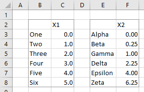
Single Block of Data

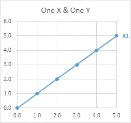
This is a fiddling case, and probably not what people are request about. But I'll cover it just for completeness.

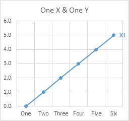
If I have a single block of data, I can select the block of data, or but a single prison cell within information technology, and Excel will build a chart using all of the data. The first column (if series are plotted past column) is used for Ten values, the remainder of the columns become the Y values, and the outset row is used for serial names.

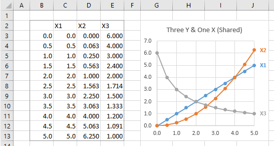
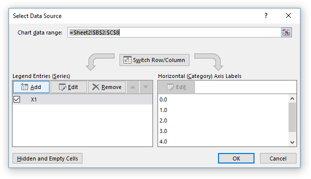
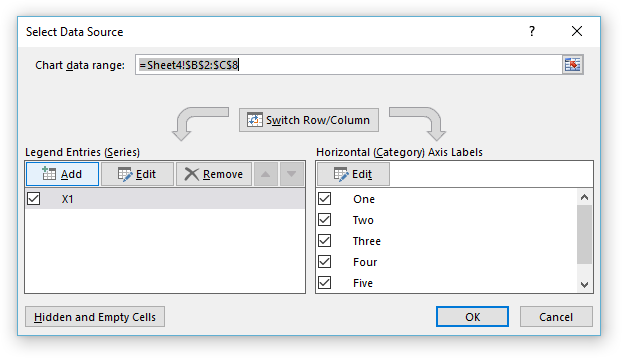
Select Series Data: If I somehow have a nautical chart that uses only function of the data, I can right click on the chart and choose Select Data, or I tin can click Select Information on the ribbon, and the Select Data Source dialog pops up. I can and then edit the Nautical chart Data Range, either by manually editing the address, or by selecting a different range, to update the chart.

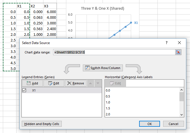
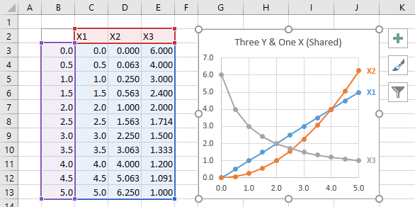
Highlighted Chart Data: But it'due south even easier to do without the dialog. If I select the chart, I tin see the nautical chart's data highlighted in the worksheet.

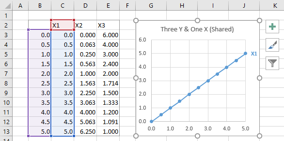
I tin can click on any of the handles on the corners of the highlighted ranges to stretch the amount of data used in the nautical chart.

Easy peasy, correct? I've written about this elementary yet powerful technique for controlling chart data in Chart Source Data Highlighting, Chart Series Data Highlighting, and Highlighted Chart Source Data.

Annotation: The default Excel chart has a fable, and I've replaced information technology with color-coded data labels on the last bespeak of each series in the nautical chart. When new serial are added, they would also be listed in the legend. In my sample charts to a higher place, I had to add the data label every time I added a new series. What a hurting, yous say? Not actually. In Peltier Tech Charts for Excel, ane of the most used features adds a label to the last bespeak of a selected series, or the last point of every serial in one or more selected charts. A relates characteristic matches the characterization color to the plotted series.

Multiple Blocks of Data

It's not every bit easy to manipulate your chart'due south information when the data resides in separate blocks of information, such equally this:

You have to start past selecting one of the blocks of information and creating the chart.

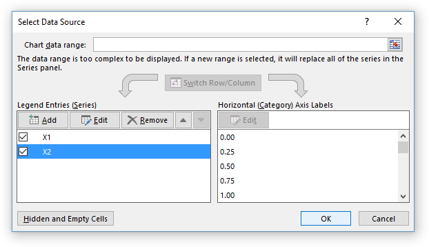
Select Series Information: Right click the chart and choose Select Data, or click on Select Information in the ribbon, to bring upwardly the Select Data Source dialog. Yous tin can't edit the Chart Data Range to include multiple blocks of information. Withal, you can add together information by clicking the Add together button higher up the list of series (which includes only the first series).

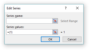
The Select Data Source dialog disappears, while a smaller Edit Series dialog pops upward, with spaces for series proper noun, 10 values, and Y values.

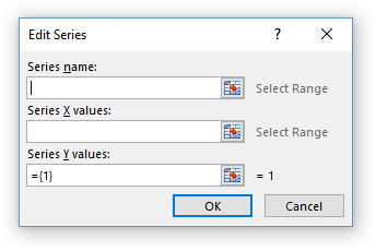
Select ranges for each of these…

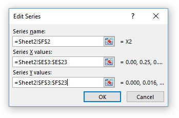
… then click OK and the new data appears as a new series in the list.

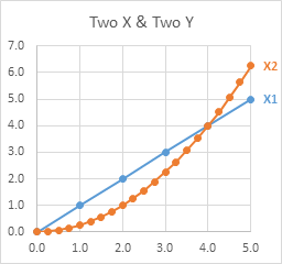
The chart now has two series. Note that in an XY Scatter chart, each series can have its own 10 values, independent of the other series in the chart.

Repeat as needed to fully populate the chart.

Not too bad, but I'm not a huge fan of the Select Data Source dialog. It just seems similar too much work. And like the expansion of data inside a single range that I started this commodity with, there's a faster and easier manner to add together data to a chart from dissimilar ranges.

Re-create – Paste Special: Select and re-create the data you desire to add to the chart, then select the nautical chart, and from the Home tab of the ribbon, click the Paste dropdown, and select Paste Special. You will exist greeted with the Paste Special dialog.

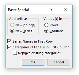
Make sure that the settings in the dialog are right: Values (Y) in rows or columns, series names in start row, categories (X labels) in first cavalcade.

The Replace Existing Categories setting would replace existing 10 values with those being pasted, which makes little sense for an XY nautical chart that already has X values divers. We'll talk about this setting when we talk over Line charts. For XY Scatter charts, I never ever check this box.

Click OK and the chart has a new series.

Copy the next range, select the chart, Paste Special.

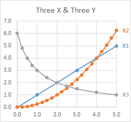
Again, in an XY Scatter nautical chart, each series can have its own X values, plotted along the same Ten axis calibration, independent of the other series in the nautical chart.

This is pretty easy. Information technology's even easier to use Paste instead of Paste Special, but sometimes Excel guesses incorrectly on those row/column, start row, first column settings, and you lot'll have to disengage the Paste and do Paste Special.

Displaying Multiple Series in a Line (Column/Area/Bar) Chart

I'1000 using Line charts here, simply the behavior of the X centrality is the same in Column and Area charts, and in Bar charts, merely y'all take to think that the Bar nautical chart'due south X axis is the vertical axis, and information technology starts at the bottom and extends upwards.

Single Block of Information

When your data is in a single block, a Line chart works just like the XY scatter chart. The beginning column (if the series information is plotted in columns) is used as Ten values, or more accurately, 10 labels; the residue of the columns are used as Y values. The get-go row is used for series names.

Multiple Blocks of Data

When there are multiple blocks of information, Line charts even so piece of work mostly the same as XY Besprinkle charts. Let's look at this simple data.

First by creating a Line chart from the first block of information.

Select Serial Data: Correct click the chart and cull Select Information from the pop-up menu, or click Select Data on the ribbon.

As before, click Add together, and the Edit Series dialog pops upwardly. There are spaces for series name and Y values.

Fill in entries for serial name and Y values, and the chart shows ii series. The original X labels remain on the chart.

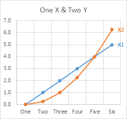
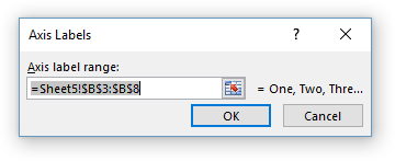
This dialog differs from the one seen when adding data to an XY Scatter chart, because there is no place for Ten values (or X labels). To alter the X labels, click the Edit push above the listing of X labels in the nautical chart. The Axis Labels dialog appears.

The reason for this is that Line charts (plus Column, Area, and Bar charts) treat 10 values differently than XY Scatter charts. XY Scatter charts care for Ten values as numerical values, and each series can accept its own independent Ten values. Line charts and their ilk treat X values as non-numeric labels, and all series in the chart apply the aforementioned 10 labels.

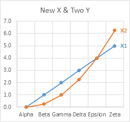
Modify the range in the Centrality Labels dialog, and all serial in the chart now use the new Ten labels.

The differences betwixt Line and XY Scatter charts can exist confusing. What is important is that the information tin can be formatted the same (markers or no markers, lines or no lines), while the X values are treated differently (numerical values in XY Besprinkle charts, non-numeric labels in Line charts).

Copy – Paste Special: Equally in XY Besprinkle charts, adding data to Line charts can exist faster and easier with Copy and Paste Special than with the Select Data dialog.

Check the settings in the dialo: Values (Y) in rows or columns, series names in first row, categories (X labels) in beginning column. If Supervene upon Existing Categories is unchecked, the original X labels will remain in the chart. Click OK to update the chart.

Although both serial are plotted against the original Ten labels, if we examine the series formulas, we run into that the original series formula contains the original X labels range ($B$3:$B$viii), while the new series formula references the new range ($E$3:$Eastward$eight).

                      =Serial(Sheet4!$C$two,Sheet4!$B$3:$B$8,Sheet4!$C$3:$C$viii,i)        

                      =SERIES(Sheet4!$F$two,Sheet4!$E$3:$E$eight,Sheet4!$F$3:$F$8,2)        

The Ten labels specified in the first series formula is what Excel uses for the chart. If we had selected only the new Y values, ignoring whatsoever new X values, and kept Categories in Kickoff Column unchecked, both series formulas would reference the aforementioned X label range.

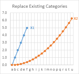
Here is what happens when we check Supplant Existing Categories.

When nosotros click OK to update the chart, the new X labels announced forth the axis. In addition, both series formulas include the new 10 label range.

This usually isn't what I want, and so I nigh never bank check Supercede Existing Categories for any nautical chart type.

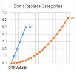
The behavior even becomes stranger when nosotros employ mismatched data ranges. The second range below has many more rows than the first.

Here is the chart if we paste special with Replace Existing Categories unchecked. Both serial use the same X labels, so the axis has plenty spaces for the longest series. Since the starting time labels are being used, these fill the first part of the axis, overlapping excessively, while the rest of the axis remains unlabeled. The beginning series is pushed to the left of the chart forth with the axis labels, since information technology simply uses a fraction of the Ten axis labels.

Here is the same chart if we paste special with Supervene upon Existing Categories checked. Both series use the new 10 labels, which fill up the entire length of the axis, and they don't overlap excessively since I wisely used one-character labels. The first series is again pushed to the left of the chart, since it has many fewer points than the 2d serial.

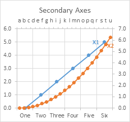
You can assign 1 series to the principal centrality and the other to the secondary centrality, and each axis volition be long enough for its labels. Beneath, the first series is plotted on the primary axis (bottom and left edges of the chart), while the second series is plotted on the secondary axis (top and right edges).

It is easier to assign the new serial to the secondary axis because I kept the Replace Existing Categories unchecked. This kept the new Ten characterization range in the serial formula even though the series was initially plotted against the original labels. When I switched the series to the secondary axis, information technology used the new X labels from the serial formula. If I had used Supercede Existing Categories, the original categories would have been removed from the original series formula, and I would have had to restore them.

I oversimplified when I stated earlier that all serial in a Line (Cavalcade, Area, Bar) nautical chart utilise the same X labels. Information technology'due south more accurate to say that all primary axis series in a Line chart use the primary axis labels, while all secondary axis serial use the secondary axis labels.

You tin can try to do a little rescaling of axes to make the chart look better. Here I set the aforementioned maximum and minimum values for primary and secondary Y axes. I also formatted the Axis Position to On Tick Marks for both primary and secondary 10 axes: "1" lines up with "a" and "Six" lines upwards with "u", and fortunately there are the right number of categories that each category on the primary scale lines upward with a category on the secondary scale ("Two" with "east", "Three" with "i", etc.). This alignment was a happy blow.

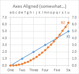
I hardly ever have a secondary 10 centrality on a line chart, since there is unremarkably no relationship between the 2 sets of labels, merely our eye insists on seeing such a relationship. I've written near this confusion acquired by Secondary Axes in Charts, even when practical in a well-meaning way.

hurtcouser.blogspot.com

Source: https://peltiertech.com/multiple-series-in-one-excel-chart/